概念
代价函数,或叫损失函数,英文为Cost Function。
假设训练样本\((x,y)\),模型为\(h\),参数为\(\theta\),则
单样本代价函数\(C(\theta)\):
任何能够衡量模型预测出来的值\(h(\theta)\)与真实值\(y\)之间的差异的函数。
多样本代价函数\(J(\theta)\):
对于多个样本,可以将所有代价函数\(C(\theta)\)的取值求均值。
获得最好的模型过程,就是得到代价函数\(J(\theta)\)的最小值,也是训练参数\(\theta\)的过程,即为
在训练参数\(\theta\)的过程中,最常用方法为梯度下降,即代价函数\(J(\theta)\)对\(\theta_1,\theta_2,…,\theta_n\)的偏导数。
其性质如下:
- 对于每种算法来说,代价函数不是唯一的;
- 代价函数是参数\(\theta\)的函数;
- 多样本代价函数\(J(\theta)\)可以用来评价模型的好坏,代价函数越小说明模型和参数越符合训练样本\((x,y)\);
- \(J(\theta)\)是一个标量;
- 最好挑选对参数\(J(\theta)\)可微的函数.
常见形式
代价函数需满足两个基本要求:
- 对模型评估的精准性
- 对参数\(J(\theta)\)可微
线性回归中的均方误差
均方误差(Mean squared error),即
- m: 训练样本的个数;
- \(h_{\theta}(x)\): 预测出的y值
- y: 原始y值,即为真实y值
- i: 第i个样本
示例
已知训练样本为\({(0,0),(1,1),(2,2),(4,4)}\)。如下图所示,很明显,其中\(y=x\)这条线为最好的模型。
模型为
取参数项\(\theta_{0}=0\).
Python下的编程
代码下载:costFunctionExam.py
# -*- coding:utf8 -*-

"""
@author: [email protected]

@date: Tue, May 23 2017

@time: 19:05:20 GMT+8
"""
import matplotlib.pyplot as plt
import numpy as np

# 都转换成列向量
X = np.array([[0, 1, 2, 4]]).T
Y = np.array([[0, 1, 2, 4]]).T

# 三个不同的theta_1值
theta1 = np.array([[0, 0]]).T
theta2 = np.array([[0, 0.5]]).T
theta3 = np.array([[0, 1]]).T

# 矩阵X的行列(m,n)
X_size = X.shape

# 创建一个(4,1)的单位矩阵
X_0 = np.ones((X_size[0], 1))

# 形成点的坐标
X_with_x0 = np.concatenate((X_0, X), axis=1)

# 两个数组点积
h1 = np.dot(X_with_x0, theta1)
h2 = np.dot(X_with_x0, theta2)
h3 = np.dot(X_with_x0, theta3)

# r:red x: x marker
plt.plot(X, Y, 'rx', label='y')
plt.title("Cost Function Example")
plt.grid(True)
plt.plot(X, h1, color='b', label='h1, theta_1=0')
plt.plot(X, h2, color='m', label='h2, theta_1=0.5')
plt.plot(X, h3, color='g', label='h3, theta_1=1')

# 坐标轴名称
plt.xlabel('X')
plt.ylabel('y/h')

# 坐标轴范围
plt.axis([-0.1, 4.5, -0.1, 4.5])
# plt.legend(loc='upper left')
plt.legend(loc='best')
plt.savefig('liner_gression_error.png', dpi=200)
plt.show()
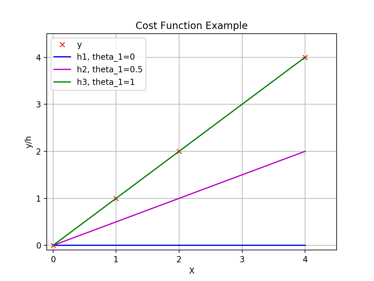
可知,不同的\(\theta_{1}\)得到不同的拟合直线,即获得以下\(J(\theta)\)的图形。
代码下载:costFunctionExam1.py
# -*- coding:utf8 -*-

"""
@author: [email protected]

@date: Tue, May 23 2017

@time: 19:05:20 GMT+8
"""

import matplotlib.pyplot as plt
import numpy as np

def calcu_cost(theta, X, Y):
    """ 计算代价函数的值

    :param theta: 斜率
    :param X: x值
    :param Y: y值
    :return: J值
    """
    m = X.shape[0]
    h = np.dot(X, theta)
    return np.dot((h - Y).T, (h - Y)) / (2 * m)


X = np.array([[0, 1, 2, 4]]).T
Y = np.array([[0, 1, 2, 4]]).T

# 从-2到4之间返回均匀间隔的数字,共101个
# theta是101*1的矩阵
theta = np.array([np.linspace(-2, 4, 101)]).T

J_list = []
for i in range(101):
    current_theta = theta[i:(i + 1)].T
    cost = calcu_cost(current_theta, X, Y)
    J_list.append(cost[0, 0])

plt.plot(theta, J_list)

plt.xlabel('theta_1')
plt.ylabel('J(theta)')
plt.title('Cost Function Example1')
plt.grid(True)
plt.savefig('cost_theta.png', dpi=200)
plt.show()
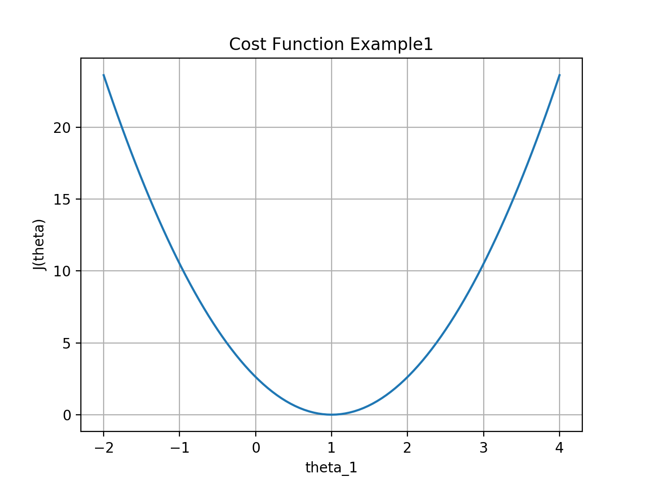
从图中轻易看出,当\(\theta=1\)时,代价函数\(J(\theta)\)取到最小值。
若取参数项\(\theta_{0}不为0\),则有两个参数。
代码下载:costFunctionExam2.py
# -*- coding:utf8 -*-

"""
@author: [email protected]

@date: Tue, May 23 2017

@time: 19:05:20 GMT+8

matplotlib version: 2.0.2
"""

import matplotlib.pyplot as plt
from mpl_toolkits.mplot3d.axes3d import Axes3D
import numpy as np


def calcu_cost(theta_0, theta_1, X, Y):
    """ 计算代价函数的值

    :param theta_0: y轴上的值
    :param theta_1: 斜率
    :param X: x值
    :param Y: y值
    :return: J值
    """
    m = X.shape[0]
    h = np.dot(X, theta_1) + theta_0
    return np.dot((h - Y).T, (h - Y)) / (2 * m)


X = np.array([[0, 1, 2, 4]]).T
Y = np.array([[0, 1, 2, 4]]).T

# 预估的点数
points_num = 41
# 点数最小值
min_point = -2
# 点数最大值
max_point = 2

# 从-2到4之间返回均匀间隔的数字,共101个
origin_theta_0 = np.array([np.linspace(min_point, max_point, points_num)]).T
origin_theta_1 = np.array([np.linspace(min_point, max_point, points_num)]).T

theta_0_list = []
theta_1_list = []

J_list = []
for i in range(points_num):
    current_theta_0 = origin_theta_0[i:(i + 1)].T
    for j in range(points_num):
        theta_0_list.append(current_theta_0[0, 0])
        current_theta_1 = origin_theta_1[j:(j + 1)].T
        theta_1_list.append(current_theta_1[0, 0])
        cost = calcu_cost(current_theta_0, current_theta_1, X, Y)
        J_list.append(cost[0, 0])

fig = plt.figure()
ax = Axes3D(fig)
ax.scatter(theta_0_list, theta_1_list, J_list, color='c')

for j in range(len(theta_0_list)):
    if J_list[j] == min(J_list):
        label_txt = 'Min J_theta(%s, %s)= %s' % (str(theta_0_list[j]), str(theta_1_list[j]), str(J_list[j]))
        ax.scatter(theta_0_list[j], theta_1_list[j], J_list[j], color='k', label=label_txt)
ax.set_xlabel('theta_0')
ax.set_ylabel('theta_1')
ax.set_zlabel('J_theta')
ax.legend(loc='upper right')
ax.view_init(30, 35)
plt.show()
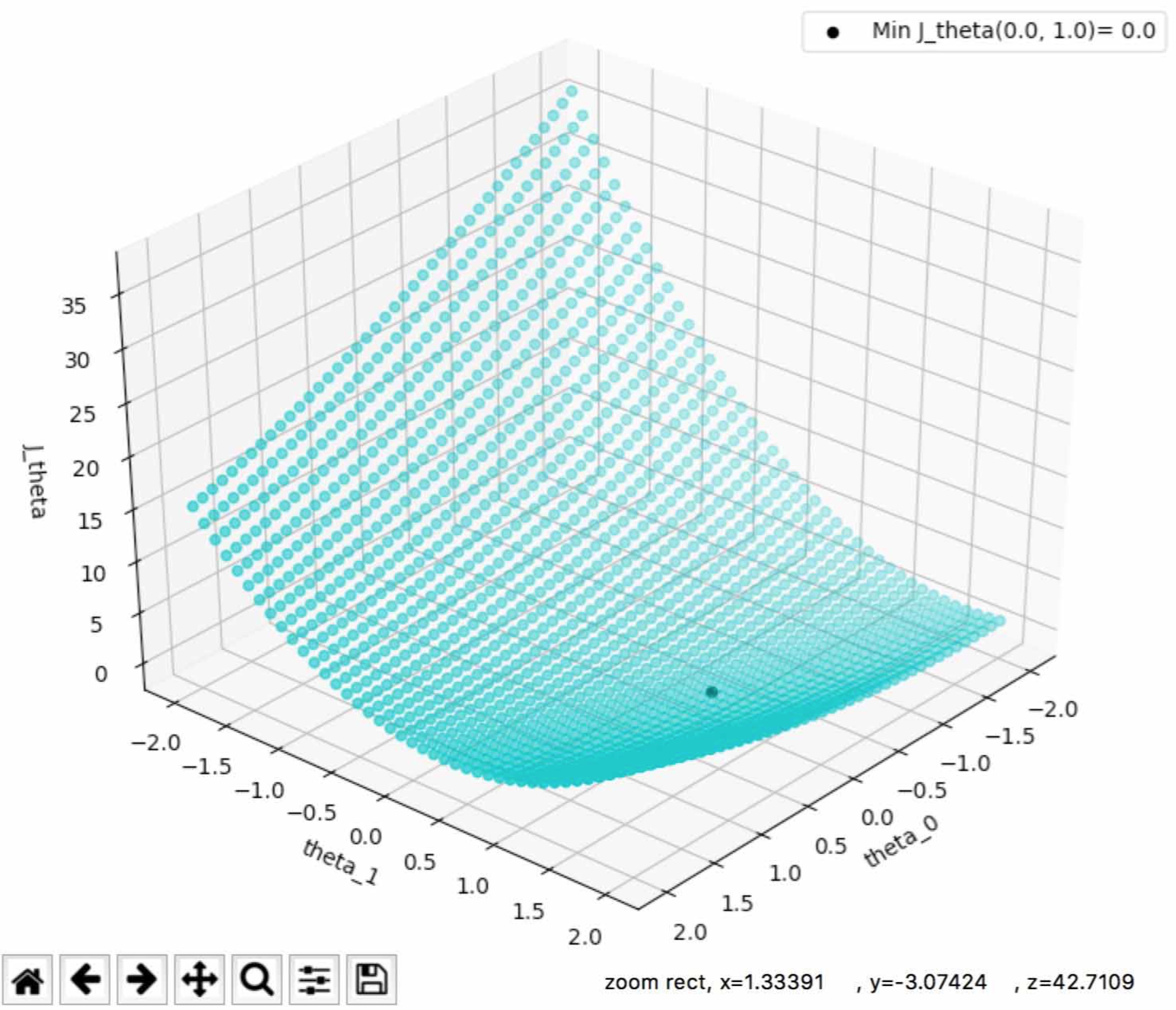
其中由于是断点,取值点数多少,最大最小值会影响到最终的结果。 例如点数为偶数时,\(J(\theta_{0}, \theta_{1})\)的最小值不为0,而是无限接近0.
Matlab下的编程
- main.m
代码下载:main.m
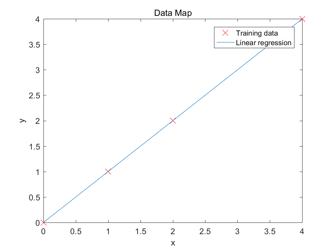
data = [0 0; 1 1; 2 2; 4 4];
x = data(:,1); y = data(:,2);
figure;
plot(x, y, 'rx', 'MarkerSize', 10);
xlabel('x'); ylabel('y');title('Data Map')
fprintf('Program paused. Press enter to continue.\n');
pause;
m = length(y);
X = [ones(m, 1), data(:,1)];
theta = zeros(2, 1);
alpha = 0.01;
iterations = 1500;
theta = GradientDescent(X, y, theta, alpha, iterations);
hold on;
plot(x, X*theta, '-')
legend('Training data', 'Linear regression')
hold off;
fprintf('the theta_0 is %f\n', theta(1,1));
fprintf('the theta_1 is %f\n', theta(2,1));
min_x=-20;
max_x=20;
num=110;
theta_1=linspace(min_x, max_x, num);
theta_0=linspace(min_x, max_x, num);
J = zeros(length(theta_0), length(theta_1));
for i = 1:num
for j = 1:num
t = [theta_0(i); theta_1(j)];
h = X * t;
J(i, j) = sum((h - y).^2) / (2 * m);
end
end
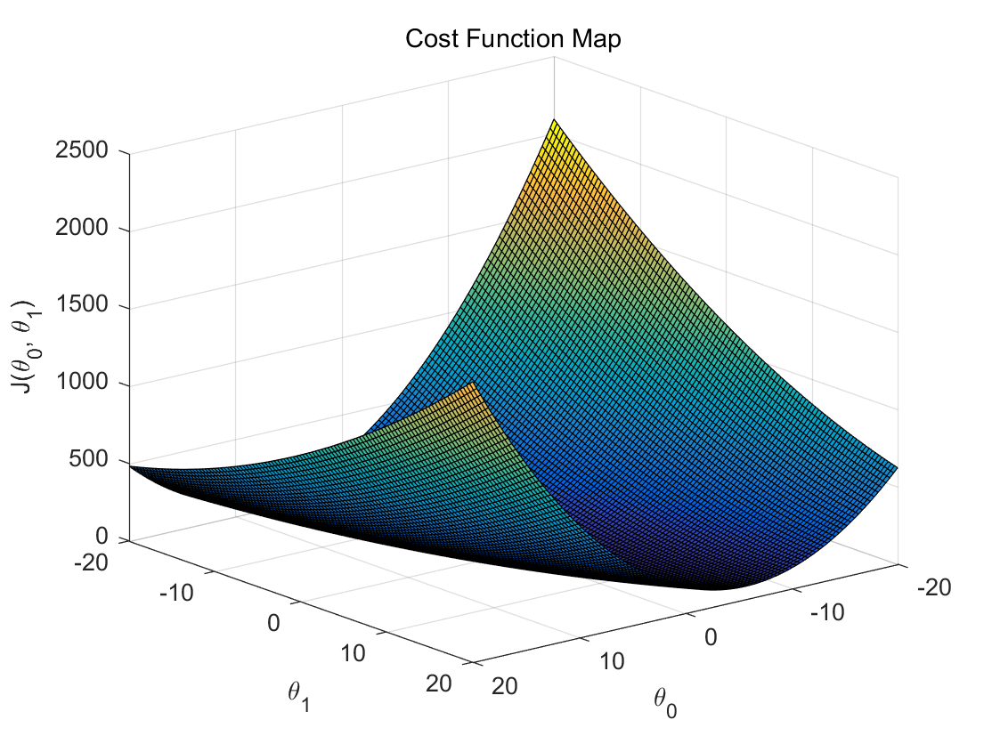
figure;
surf(theta_0, theta_1, J);
xlabel('\theta_0');ylabel('\theta_1');zlabel('J(\theta_0, \theta_1)')
title('Cost Function Map')
[b, c] = find(J==min(J(:)));
disp([b, c]);
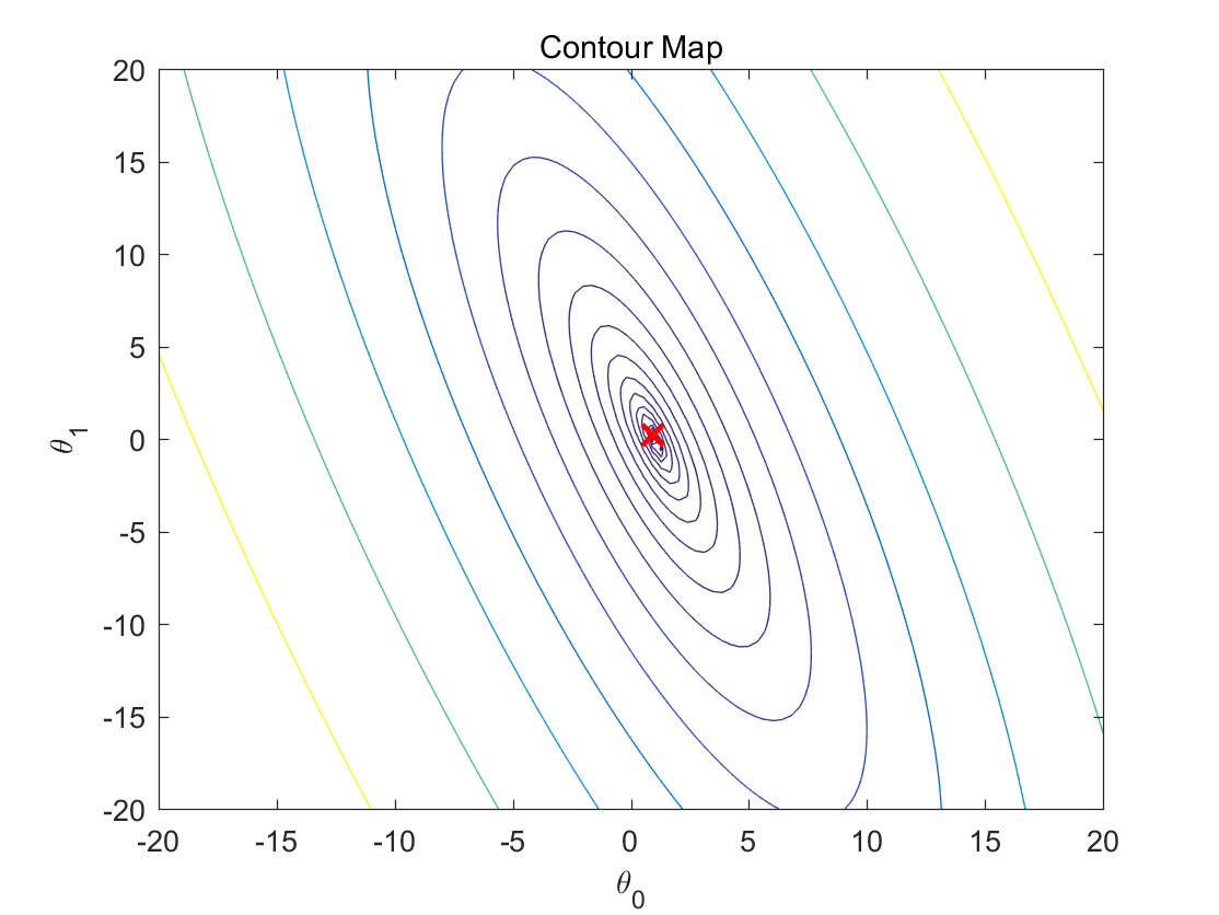
figure;
contour(theta_0, theta_1, J, logspace(-2, 3, 20))
xlabel('\theta_0'); ylabel('\theta_1');
title('Contour Map')
hold on;
plot(theta_0(c), theta_1(b), 'rx', 'MarkerSize', 10, 'LineWidth', 2);
hold off;
- CostFunction.m
代码下载:CostFunction.m
function J = CostFunction(X, y, theta)

m = length(y);
J = 0;

h = X * theta;
J = sum((h - y).^2) / (2 * m);

end
- GradientDescent.m
代码下载:GradientDescent.m
function [theta, J_history] = GradientDescent(X, y, theta, alpha, iterations_num)

m = length(y);
J_history = zeros(iterations_num, 1);

for iter = 1:iterations_num
    h = X * theta;
    t = [0; 0];
    for i = 1:m
        t = t + (h(i) - y(i)) * X(i,:)';
    end

    theta = theta - alpha * (1 / m) * t;

    J_history(iter) = CostFunction(X, y, theta);
end

end
结果如下:
梯度下降算法在代价函数上的应用
代价函数
梯度下降算法
重复直至收敛:
则:
当\(j=0\)时,
当\(j=1\)时,
综上所述,
Troubleshooting
Mac上的安装matplotlib问题
Mac上面pip install matplotlib后出现:
<<'COMMENT'
Traceback (most recent call last):
 File "2.py", line 2, in <module>    import pylab  File "/Users/twcn/.pyenv/versions/3.5.1/lib/python3.5/site-packages/pylab.py", line 1, in <module>
 from matplotlib.pylab import *  File "/Users/twcn/.pyenv/versions/3.5.1/lib/python3.5/site-packages/matplotlib/pylab.py", line 274, in <module>
 from matplotlib.pyplot import *  File "/Users/twcn/.pyenv/versions/3.5.1/lib/python3.5/site-packages/matplotlib/pyplot.py", line 114, in <module>    _backend_mod, new_figure_manager, draw_if_interactive, _show = pylab_setup()  File "/Users/twcn/.pyenv/versions/3.5.1/lib/python3.5/site-packages/matplotlib/backends/__init__.py", line 32, in pylab_setup    globals(),locals(),[backend_name],0)  File "/Users/twcn/.pyenv/versions/3.5.1/lib/python3.5/site-packages/matplotlib/backends/backend_macosx.py", line 24, in <module>
 from matplotlib.backends import _macosxRuntimeError: Python is not installed as a framework. The Mac OS X backend will not be able to function correctly if Python is not installed as a framework. See the Python documentation for more information on installing Python as a framework on Mac OS X. Please either reinstall Python as a framework, or try one of the other backends. If you are Working with Matplotlib in a virtual enviroment see 'Working with Matplotlib in Virtual environments' in the Matplotlib FAQ
COMMENT
解决方法:
cd ~/.matplotlib
touch matplotlibrc
cat >> matplotlibrc <<EOF
backend: TkAgg
EOF
参考博文
- MathJax basic tutorial and quick reference
- 基本数学公式语法MathJax
- numpy数组初探
- tf.concat与numpy.concatenate
- 机器学习代价函数cost-function
 本作品由陈健采用知识共享署名-非商业性使用-相同方式共享 4.0 国际许可协议进行许可。